Showcasing of AMBER utilizing synthetic neutron scattering data
[1]:
import numpy as np
from AMBER.background import background
import matplotlib.pyplot as plt
Generate signal data
The data for this tutorial is generated using the expected neutron scattering signal in an inelastic exmperiment measuring MnF\(_2\). The dispersion relation, i.e. the energy at a give (H,K,L) position is given by the analytical formula Yamany et al. 2010:
In the above \(J_1\), \(J_2\), and \(D\) are the magnetic coupling strengths and single-ion anisotropy which determine the amplitude of the dispersion. The parameters \(S = 5/2\), \(z_1 = 2\), and \(z_2 = 8\) corresponds the the size of the magnetic spin, and the number of nearest and next-nearest neighbours in the MnF\(_2\) lattice.
From the above equation, the imporant fact is that it depends on the 3D vector \(Q = (H,K,L)\). For simplicity, we assume that \(K\) is zero and thus reduce the data to 3D, i.e. \((H,L,\omega)\)
Due to how neutron scattering experiments function, the above dispersion will not be infinitely thin but rather extended. Here, this is replicated by a simple gaussian smearing along \(\omega\)
[2]:
# Define parameters, dispersion, and Smearing
S = 5/2
z1 = 2
z2 = 8

def SpinWave(Q,J1,J2,D):
    return np.sqrt(np.power(2*S*z2*J2+D+2*z1*S*J1*np.sin(Q[2]*np.pi)**2,2.0)-

            np.power(2*S*z2*J2*np.cos(Q[0]*np.pi)*np.cos(Q[1]*np.pi)*np.cos(Q[2]*np.pi),2.0))

def Intensity(H,K,L,E):
    sigmaE = 0.25
    omega = SpinWave(np.array([H,K,L]),  J1=0.0354,J2=0.1499,D=0.131 )
    I = np.exp(-np.power(omega-E,2.0)/(2*sigmaE**2))

    return I
Define 3D grid domain
The input to AMBER is a 3D cube of intensities which is define below
[3]:
# Data will ge simulated along H and L but with K = 0

h = np.linspace(-0.1,2.1,101)
k = 0
l = np.linspace(-0.1,2.1,101)

# Choose a sufficient energy range
e = np.linspace(0.5,8,61)

# Generate the grid upon which the dispersion is calculated

H,L,E = np.meshgrid(h,l,e)
K = np.zeros_like(H)

# Intensities are calculated with the smearing and scaled
I = 30*Intensity(H,K,L,E)

# Poisson noice is added to the intensity
I = np.random.poisson(I).astype(float)
Introduction of NaN-values
Triple axis instruments cannot measure all lengths of \(Q\). this we can mimic by exchaning the intensity at these points by NaNs
[4]:
QLength = np.linalg.norm([H,L],axis=0)

I[QLength<0.35] = np.nan
I[QLength>2.5] = np.nan
Add background
The main feature of AMBER is the background segmentation, which requires the data to have a background. As describe in the article, background is assumed to:
Rotation independence of the background.
Smooth change of background along energy and \(|\vec{Q}|\).
The signal is sparse but continuous in energy and \(|\vec{Q}|\).
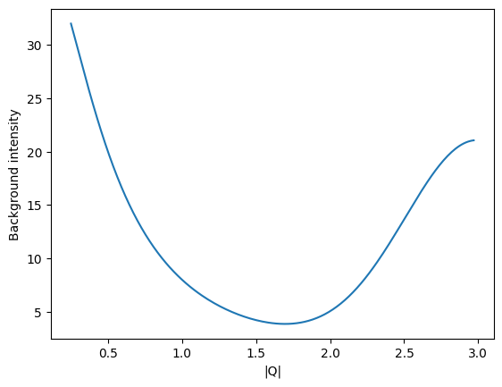
In the following, a background is generated with a higher amplitude for low and high \(|\vec{Q}|\) mimicing instrumental background artefacts from triple axis neutron experiments - these corresponds to the direct beam contribution and to increased background at larger scattering angles.
[5]:
# Background definition
def background_simulation(q,amplitude,gamma,mu,amplitude2,gamma2):
    return amplitude*((gamma/(q**2+gamma**2))+amplitude2*np.exp(-np.power(q-mu,2.0)/(2*gamma2**2)))


Q = np.linalg.norm([H,K,L],axis=0)

# Choose suitable valies
gamma = 0.5
mu = 3.0
amplitude = 20
amplitude2 = 1.0
gamma2 = 0.5

# Generate an example of the background for visual inspection
q = np.linspace(0.25,Q.max(),201)
bg_test = background_simulation(q,amplitude,gamma,mu,amplitude2,gamma2)

# display background amplitude
fig,ax = plt.subplots()
ax.plot(q,bg_test)
ax.set_xlabel('|Q|')
ax.set_ylabel('Background intensity')


## Add background to data
bg_tmp = background_simulation(Q,amplitude,gamma,mu,amplitude2,gamma2)

I+=np.random.poisson(bg_tmp)
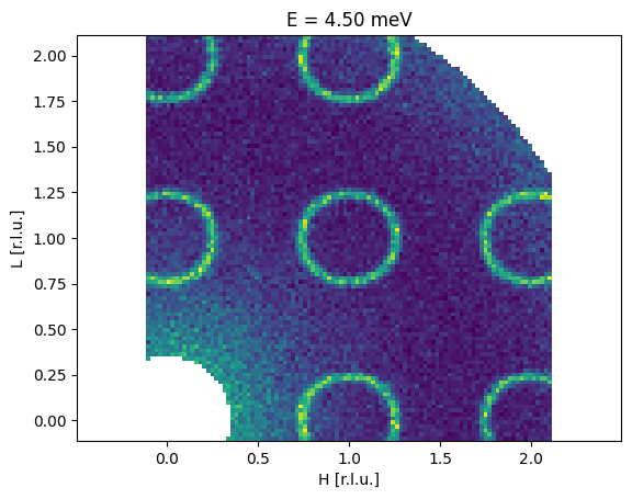
Plot a constant energy plot
The now background affected data is plotted to show a “before” picture. This is done by choosing a specific energy (\(\omega \sim 4.5\) meV) and plotting the intensity as a color map
[6]:
fig,ax = plt.subplots()

# Find the closest energy slice
energy = 4.5
EIdx = np.argmin(np.abs(E-energy))
ax.pcolormesh(H[:, :, EIdx], L[:, :, EIdx], I[:, :, EIdx], vmin=0, vmax = 50)

ax.axis('equal')
ax.set_title('E = {:.2f} meV'.format(e[EIdx]))
ax.set_xlabel('H [r.l.u.]')
ax.set_ylabel('L [r.l.u.]')
[6]:
Text(0, 0.5, 'L [r.l.u.]')
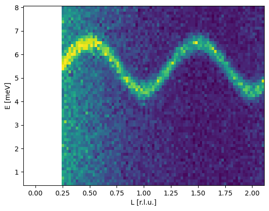
Plot a constant H map
[7]:
fig,ax = plt.subplots()

h_value = 0.25
HIdx = np.argmin(np.abs(h-h_value))
ax.pcolormesh(L[:, HIdx, :],E[:, HIdx, :],I[:, HIdx, :], vmin=0, vmax=50)

ax.set_xlabel('L [r.l.u.]')
ax.set_ylabel('E [meV]')
[7]:
Text(0, 0.5, 'E [meV]')
Run denoising algorithm
[8]:
# Initialize the AMBER background object

AMBER = background(dtype=np.float32)

# Set the grid sizes
AMBER.set_gridcell_size(dqx = 0.022, dqy = 0.022, dE = 0.125)

# Alternatively these can be set from the h, l, and e arrays like
# AMBER.set_volume_from_limits([h[0],l[0],e[0]],[h[-1],l[-1],e[-1]],)

# Input the data
AMBER.set_binned_data(h, l, e, I)

bins = int((q.max()-q.min())/0.022)

# define maximum radius and number of bins
AMBER.set_radial_bins(q.max(),n_bins=bins)
Set algorithm parameters (\(\lambda, \beta, \mu\))
lambda and mu will be determined as described in the paper and we select beta using cross validation
beta_ is selected using cross validation, i.e. mask out the top q quantile of intensity. The beta value for the lowest Root-Mean-Square-Error is then chosen
[9]:
lambda_tmp = AMBER.MAD_lambda()
mu_tmp = AMBER.mu_estimator()


beta_range_tmp = np.array([0.1,1.0,10.0,100.0,200.0,300.0,400.0,500.0])
rmse = AMBER.cross_validation(q=0.3,beta_range= beta_range_tmp, lambda_=lambda_tmp, mu_=mu_tmp,n_epochs=15,verbose=False)


beta_tmp = beta_range_tmp[np.argmin(rmse)]
Test - ( 0.1 )
RMSE - ( 4.4478 0.1 55.50269024150275 ) :  3.486001
Test - ( 1.0 )
RMSE - ( 4.4478 1.0 55.50269024150275 ) :  3.4850485
Test - ( 10.0 )
RMSE - ( 4.4478 10.0 55.50269024150275 ) :  3.47741
Test - ( 100.0 )
RMSE - ( 4.4478 100.0 55.50269024150275 ) :  3.4501917
Test - ( 200.0 )
RMSE - ( 4.4478 200.0 55.50269024150275 ) :  3.4432225
Test - ( 300.0 )
RMSE - ( 4.4478 300.0 55.50269024150275 ) :  3.4426384
Test - ( 400.0 )
RMSE - ( 4.4478 400.0 55.50269024150275 ) :  3.4448829
Test - ( 500.0 )
RMSE - ( 4.4478 500.0 55.50269024150275 ) :  3.4486284
Run the denoising algorithm using the parameters obtained using the heuristic
[10]:
# set number of epochs
n_epochs = 20

AMBER.denoising(AMBER.Ygrid,lambda_tmp,beta_tmp,mu_tmp,n_epochs,verbose=True)
 Iteration  1
 Loss function:  24616092.0
 Iteration  2
 Loss function:  18311960.0
 Iteration  3
 Loss function:  15576615.0
 Iteration  4
 Loss function:  14319358.0
 Iteration  5
 Loss function:  13718133.0
 Iteration  6
 Loss function:  13445899.0
 Iteration  7
 Loss function:  13333092.0
 Iteration  8
 Loss function:  13288917.0
 Iteration  9
 Loss function:  13271952.0
 Iteration  10
 Loss function:  13265445.0
 Iteration  11
 Loss function:  13262938.0
 Iteration  12
 Loss function:  13261957.0
 Iteration  13
 Loss function:  13261567.0
 Iteration  14
 Loss function:  13261418.0
 Iteration  15
 Loss function:  13261355.0
 Iteration  16
 Loss function:  13261332.0
 Iteration  17
 Loss function:  13261326.0
 Iteration  18
 Loss function:  13261322.0
Compute substracted signal
[11]:
# The subtracted signal is given by

Y_sub = AMBER.Ygrid - AMBER.b_grid
Y_back = AMBER.b_grid

# reshape the data to fit
Y_sub = Y_sub.reshape(AMBER.E_size,AMBER.Qx_size,AMBER.Qy_size).T
Y_back = Y_back.reshape(AMBER.E_size,AMBER.Qx_size,AMBER.Qy_size).T

# reshape the observation
Y_obs =  AMBER.Ygrid.reshape(AMBER.E_size,AMBER.Qx_size,AMBER.Qy_size).T
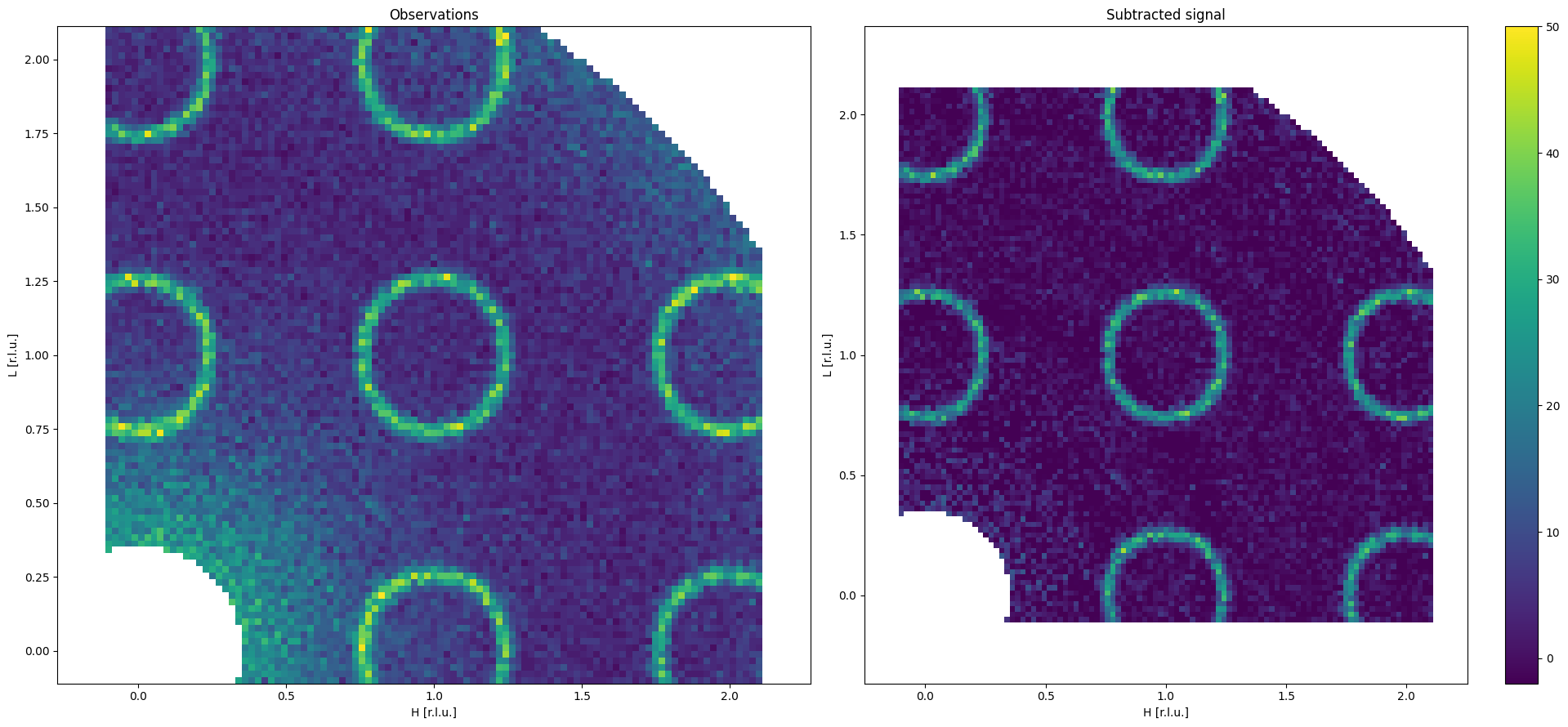
Display substracted signal
[12]:
# reshape the observation
Y_obs =  AMBER.Ygrid.reshape(AMBER.E_size,AMBER.Qx_size,AMBER.Qy_size).T


fig0 = plt.figure(figsize=(20, 9))

# Plot 1: Observations Y
ax0 = fig0.add_subplot(1, 2, 1)

energy = 4.5
EIdx = np.argmin(np.abs(E-energy))
ax0.pcolormesh(H[:,:,EIdx],L[:,:,EIdx],Y_obs[:,:,EIdx],vmin=-2,vmax=50)

ax0.axis('equal')
ax0.set_xlabel('H [r.l.u.]')
ax0.set_ylabel('L [r.l.u.]')
ax0.set_title('Observations')

# Plot 2: Subtracted Y
ax1 = fig0.add_subplot(1, 2, 2)

energy = 4.5
EIdx = np.argmin(np.abs(E-energy))
p = ax1.pcolormesh(H[:,:,EIdx],L[:,:,EIdx],Y_sub[:,:,EIdx],vmin=-2,vmax=50)

ax1.axis('equal')
ax1.set_xlabel('H [r.l.u.]')
ax1.set_ylabel('L [r.l.u.]')
ax1.set_title('Subtracted signal')

fig0.colorbar(p)
plt.tight_layout()
plt.show()
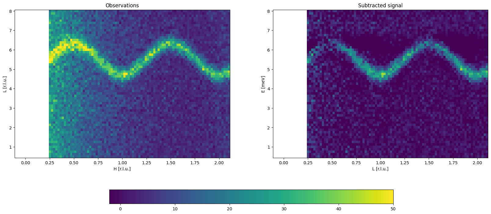
[21]:
fig0,axx = plt.subplots(figsize=(20, 9),ncols=2,nrows=1)

# Plot 1: Observations Y

ax0 = axx[0]

h_value = 0.25
HIdx = np.argmin(np.abs(h-h_value))
ax0.pcolormesh(L[:,HIdx,:],E[:,HIdx,:],Y_obs[:,HIdx,:],vmin=-2,vmax=50)

ax0.set_xlabel('H [r.l.u.]')
ax0.set_ylabel('L [r.l.u.]')
ax0.set_title('Observations')

# Plot 2: Subtracted Y
ax1 = axx[1]


HIdx = np.argmin(np.abs(h-h_value))
p = ax1.pcolormesh(L[:,HIdx,:],E[:,HIdx,:],Y_sub[:,HIdx,:],vmin=-2,vmax=50)

ax1.set_xlabel('L [r.l.u.]')
ax1.set_ylabel('E [meV]')
ax1.set_title('Subtracted signal')


fig0.colorbar(p,ax =axx, shrink=0.2, location='bottom')

#plt.tight_layout()
plt.show()
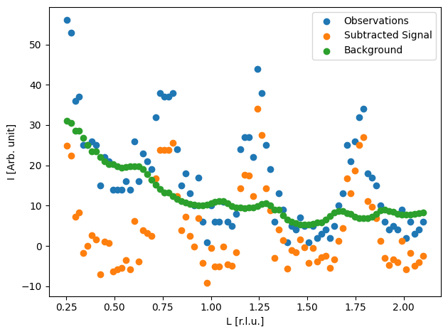
Compare the signal with the subtracted signal in a 1D cut
[14]:
fig0 = plt.figure()

# Plot 1: Observations Y
ax0 = fig0.add_subplot(1, 1, 1)

h_value = 0.25
e_value = 5.5 # meV
EIdx = np.argmin(np.abs(e-e_value))
HIdx = np.argmin(np.abs(h-h_value))
ax0.scatter(L[:,HIdx,EIdx],Y_obs[:,HIdx,EIdx],label='Observations')
ax0.scatter(L[:,HIdx,EIdx],Y_sub[:,HIdx,EIdx],label='Subtracted Signal')
ax0.scatter(L[:,HIdx,EIdx],Y_back[:,HIdx,EIdx],label='Background')


ax0.set_xlabel('L [r.l.u.]')
ax0.set_ylabel('I [Arb. unit]')
ax0.legend()


plt.tight_layout()
plt.show()